Back to Code and Software Demo

Python – Stochastic Repressilator Gene Network Using the Gillespie Algorithm

Goal

The goal of this simulation is to model a stochastic repressilator gene network using the Gillespie SSA (Stochastic Simulation Algorithm). Unlike deterministic differential equation models, this implementation captures molecular noise and random fluctuations in gene expression at the single-cell scale. The objective is to observe how oscillatory behavior in mRNA (Mi) and protein (Pi) levels can emerge purely from stochastic reaction dynamics within a three-gene inhibitory loop.

Engineering Approach and Tools

The biological system is encoded as a reaction transition matrix, where each row corresponds to a chemical reaction and each column represents a molecular species (active/inactive gene states, mRNA, proteins). At each simulation step, reaction propensities are computed based on kinetic parameters such as transcription, translation, repression, and degradation rates. The Gillespie algorithm is then used to randomly select the next reaction and its stochastic time increment using exponential sampling. The system state evolves step-by-step, and trajectories for gene state switching (Ga/Gi), mRNA synthesis (Mi), and protein production (Pi) are visualized using matplotlib.

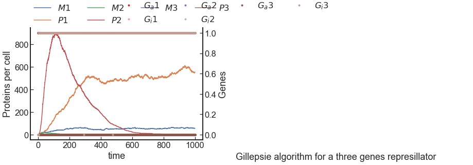
Execution Behavior and Output Interpretation

The execution produces clear stochastic oscillations in the expression levels of M1, M2, M3 and P1, P2, P3. These oscillations emerge without any deterministic enforcement, driven solely by intrinsic biochemical noise. The plots reveal alternating repression and activation cycles across the three genes, confirming that stochasticity alone can generate oscillatory gene expression patterns in a minimalist feedback network. This behavior closely aligns with biological observations where noise is not a disturbance, but a fundamental driver of dynamic regulation in living systems.

Gillespie Simulation Output

Implementation Steps

Imports
# Author: Hamza Bendahmane import numpy as np import seaborn as sns import matplotlib.pyplot as plt import warnings warnings.filterwarnings('ignore')
Definition of Rate Constants
# Author: Hamza Bendahmane ki1 = ki2 = ki3 = 0.1 kM1 = kM2 = kM3 = 5.0 kP1 = 1.0 kP2 = 10.0 kP3 = 100.0 dM1 = dM2 = dM3 = 0.1 dP1 = dP2 = dP3 = 0.1 ka1 = ka2 = ka3 = 0.01
Codify Rules in a Matrix (shape = rules x species)
# Author: Hamza Bendahmane # Ga1 Gi1 M1 P1 Ga2 Gi2 M2 P2 Ga3 Gi3 M3 P3 matrix = [[ 0, 0, 0, -2, -1, 1, 0, 0, 0, 0, 0, 0], #2P1+Ga2->Gi2 [ 0, 0, 0, 0, 0, 0, 0, -2, -1, 1, 0, 0], #2P2+Ga3->Gi3 [-1, 1, 0, 0, 0, 0, 0, 0, 0, 0, 0, -2], #2P3+Ga1->Gi1 [ 0, 0, 1, 0, 0, 0, 0, 0, 0, 0, 0, 0], #Ga1->Ga1+M1 [ 0, 0, 0, 0, 0, 0, 2, 0, 0, 0, 0, 0], #Ga2->Ga2+M2 [ 0, 0, 0, 0, 0, 0, 0, 0, 0, 0, 1, 0], #Ga3->Ga3+M3 [ 0, 0, 0, 1, 0, 0, 0, 0, 0, 0, 0, 0], #M1->M1+P1 [ 0, 0, 0, 0, 0, 0, 0, 1, 0, 0, 0, 0], #M2->M2+P2 [ 0, 0, 0, 0, 0, 0, 0, 0, 0, 0, 0, 1], #M3->M3+P3 [ 0, 0, -1, 0, 0, 0, 0, 0, 0, 0, 0, 0], #M1->0 [ 0, 0, 0, 0, 0, 0,-1, 0, 0, 0, 0, 0], #M2->0 [ 0, 0, 0, 0, 0, 0, 0, 0, 0, 0, -1, 0], #M3->0 [ 0, 0, 0, -1, 0, 0, 0, 0, 0, 0, 0, 0], #P1->0 [ 0, 0, 0, 0, 0, 0, 0, -1, 0, 0, 0, 0], #P2->0 [ 0, 0, 0, 0, 0, 0, 0, 0, 0, 0, 0, -1], #P3->0 [ 1,-1, 0, 0, 0, 0, 0, 0, 0, 0, 0, 0], #Gi1->Ga1 [ 0, 0, 0, 0, 1,-1, 0, 0, 0, 0, 0, 0], #Gi2->Ga2 [ 0, 0, 0, 0, 0, 0, 0, 0, 1,-1, 0, 0]] #Gi3->Ga3
Definition of Propensities
# Author: Hamza Bendahmane def propensities(species, ki1,kM1,kP1,dM1,dP1,ka1, ki2,kM2,kP2,dM2,dP2,ka2, ki3,kM3,kP3,dM3,dP3,ka3): Ga1, Gi1, M1, P1, Ga2, Gi2, M2, P2, Ga3, Gi3, M3, P3 = species prop = np.zeros(18) prop[0] = ki2*Ga2*(P1**2) # 2P1+Ga2->Gi2 prop[1] = ki3*Ga3*(P2**2) # 2P2+Ga3->Gi3 prop[2] = ki1*Ga1*(P3**2) # 2P3+Ga1->Gi1 prop[3] = kM1*Ga1 prop[4] = kM2*Ga2 prop[5] = kM3*Ga3 prop[6] = kP1*M1 prop[7] = kP2*M2 prop[8] = kP3*M3 prop[9] = dM1*M1 prop[10]= dM2*M2 prop[11]= dM3*M3 prop[12]= dP1*P1 prop[13]= dP2*P2 prop[14]= dP3*P3 prop[15]= ka1*Gi1 prop[16]= ka2*Gi2 prop[17]= ka3*Gi3 return prop
Update Species
# Author: Hamza Bendahmane def update_species_compact(species, rule): species = np.asarray(species) + np.asarray(matrix[rule]) return list(species)
Gillespie SSA Simulation
# Author: Hamza Bendahmane # Initialization species = [1,0,0,0, 1,0,0,0, 1,0,0,0] # Ga1,Gi1,M1,P1,Ga2,... t = 0 tstop = 1000 state = [] time = [] while t < tstop: state.append(species) time.append(t) prop = propensities(species, ki1,kM1,kP1,dM1,dP1,ka1, ki2,kM2,kP2,dM2,dP2,ka2, ki3,kM3,kP3,dM3,dP3,ka3) T = np.random.exponential(scale=10/prop) rule = np.argsort(T)[0] species = update_species_compact(species, rule) t += np.sort(T)[0] state = np.asarray(state) time = np.asarray(time) sns.set(style="ticks", font_scale=1.5, rc={'axes.linewidth':2, "axes.spines.right":True, "axes.spines.top":False, 'xtick.direction':'in','ytick.direction':'in'}) ax1 = plt.gca() ax1.plot(time, state[:,2], c=sns.color_palette()[0], label='M1') ax1.plot(time, state[:,3], c=sns.color_palette()[1], label='P1') ax1.plot(time, state[:,6], c=sns.color_palette()[2], label='M2') ax1.plot(time, state[:,7], c=sns.color_palette()[3], label='P2') ax1.plot(time, state[:,10], c=sns.color_palette()[4], label='M3') ax1.plot(time, state[:,11], c=sns.color_palette()[5], label='P3') plt.legend(loc=(0.0, 1), ncol=4, frameon=False) ax1.set_xlabel("time") ax1.set_ylabel("Proteins per cell") ax2 = ax1.twinx() ax2.plot(time, state[:,0], '.', c=sns.color_palette("tab20",20)[6], label='Ga1') ax2.plot(time, state[:,1], '.', c=sns.color_palette("tab20",20)[7], label='Gi1') ax2.plot(time, state[:,4], '.', c=sns.color_palette("tab20",20)[8], label='Ga2') ax2.plot(time, state[:,5], '.', c=sns.color_palette("tab20",20)[9], label='Gi2') ax2.plot(time, state[:,8], '.', c=sns.color_palette("tab20",20)[10], label='Ga3') ax2.plot(time, state[:,9], '.', c=sns.color_palette("tab20",20)[11], label='Gi3') plt.legend(loc=(0.5, 1), ncol=4, frameon=False) plt.figtext(1.5, 0.01, 'Gillespie algorithm for a three genes repressilator', ha='center', va='center') ax2.set_ylabel("Genes") plt.show()
© 2025 – Hamza Bendahmane. All rights reserved.